Introduction to R and RStudio

Learning Objectives

Following this assignment students should be able to:

execute simple math in the R console

assign and manipulate variables

use built-in functions for math and stats

understand the assignment and execute flow of an R script

understand the vector and data frame object structures

assign, subset, and manipulate data in a vector

execute vector algebra

import data frames and interact with columns as vectors

Reading

Topics

R & RStudio
Expressions & Variables
Types
Errors
Vectors & Data Frames
Importing Data
Readable Code

Readings

Lecture Notes

Exercises

Basic Expressions (10 pts)

Think about what value each of the following expressions will return? Check your answers using the R Console by typing each expression into the console on the line marked > and pressing enter.
1. 2 - 10
2. 3 * 5
3. 9 / 2
4. 5 - 3 * 2
5. (5 - 3) * 2
6. 4 ^ 2
7. 8 / 2 ^ 2
Did any of the results surprise you? If so, then might have run in to some order of operations confusion. The order of operators for math in R are the same as for mathematics more generally.

Now turn this set of expressions into a program that you can save by using an R script. For each expression add one line to the script. Run the script in the console to display the answer to the screen. If you are using RStudio, you can click the Run button in the top-right corner of the editor or use Ctrl+Enter (Windows & Linux) or Command+Enter (Mac) to run the line or selection of code directly from your script. You can run the entire script by clicking the arrow next to Source and selecting Source with Echo or by using Ctrl+Shift+Enter (Windows & Linux) or Command+Shift+Enter (Mac).

To tell someone reading the code what this section of the code is about, add a comment line that says ‘Exercise 1’ before the code that answers the exercise. Comments in R are added by adding the # sign. Anything after a # sign on the same line is ignored when the program is run. So, the start of your program should look something like:
```
# Exercise 1
2-10
```
[click here for output]
Basic Variables (10 pts)

Here is a small program that converts a mass in kilograms to a mass in grams and then prints out the resulting value.
```
mass_kg <- 2.62
mass_g <- mass_kg * 1000
mass_g
```
Modify this code to create a variable that stores a body mass in pounds and assign it a value of 3.5 (about the right size for a Desert Cottontail Rabbit – Sylvilagus audubonii). Convert this value to kilograms. There are approximately 2.2046 lbs in a kilogram, so divide the variable storing the weight in pounds by 2.2046 and store this value in a new variable for storing mass in kilograms. Print the value of the new variable to the screen.
[click here for output]
More Variables (10 pts)

Calculate a total biomass in grams for 3 white-throated woodrats (Neotoma albigula) and then convert it to kilograms. The total biomass is three times the average size of a single individual. An average individual weighs 250 grams.
1. Add a new section to your R script starting with a comment.
2. Create a variable grams and assign it the mass of a single Neotoma albigula.
3. Create a variable number and assign it the number of individuals.
4. Create a variable biomass and assign it a value by multiplying the grams and number variables together.
5. Convert the value of biomass into kilograms (there are 1000 grams in a kilogram so divide by 1000) and assign this value to a new variable.
6. Print the final answer to the screen.
Are the variable names grams, number, and biomass the best choice? If we came back to the code for this assignment in two weeks would we be able to remember what these variables were referring to and therefore what was going on in the code? The variable name biomass is also kind of long. If we had to type it many times it would be faster just to type b. We could also use really descriptive alternatives like individual_mass_in_grams. Or we would compromise and abbreviate this or leave out some of the words to make it shorter (e.g., indiv_mass_g).

Think about good variable names and then rename the variables in your program to what you find most useful. Make sure your code still runs properly after you’ve changed the names.
[click here for output]
Built-in Functions (10 pts)

A built-in function is one that you don’t need to install and load a package to use. To learn how to use a function you can use the help() function or the Help tab in RStudio. help() takes one parameter, the name of the function that you want information about (e.g., help(abs)) or type the name into the search box on the Help tab. Familiarize yourself with the built-in functions abs(), round(), sqrt(), tolower(), and toupper(). Use these built-in functions to print the following items:
1. The absolute value of -15.5.
2. 4.483847 rounded to one decimal place. The function round() takes two arguments, the number to be rounded and the number of decimal places.
3. 3.8 rounded to the nearest integer. You don’t have to specify the number of decimal places in this case if you don’t want to, because round() will default to using 0 if the second argument is not provided. Look at help(round) or ?round to see how this is indicated.
4. "species" in all capital letters.
5. "SPECIES" in all lower case letters.
6. Assign the value of the square root of 2.6 to a variable. Then round the variable you’ve created to 2 decimal places and assign it to another variable. Print out the rounded value.
Challenge: Do the same thing as task 6 (immediately above), but instead of creating the intermediate variable, perform both the square root and the round on a single line by putting the sqrt() call inside the round() call.
[click here for output]
Modify the Code (10 pts)

The following code estimates the total net primary productivity (NPP) per day for two sites. It does this by multiplying the grams of carbon produced in a single square meter per day by the total area of the site. It then prints the daily NPP for each site.
```
site1_g_carbon_m2_day <- 5
site2_g_carbon_m2_day <- 2.3
site1_area_m2 <- 200
site2_area_m2 <- 450
site1_npp_day <- site1_g_carbon_m2_day * site1_area_m2
site2_npp_day <- site2_g_carbon_m2_day * site2_area_m2
site1_npp_day
site2_npp_day
```
Modify the code to produce the following items and print them out after the daily NPP values (the ones currently printed by the code):
1. The sum of the total daily NPP for the two sites combined.
2. The difference between the daily NPP for the two sites. We only want an absolute difference, so use abs() function to make sure the number is positive.
3. The total NPP over a year for the two sites combined (the sum of the total daily NPP values multiplied by 365).
[click here for output]
Code Shuffle (10 pts)

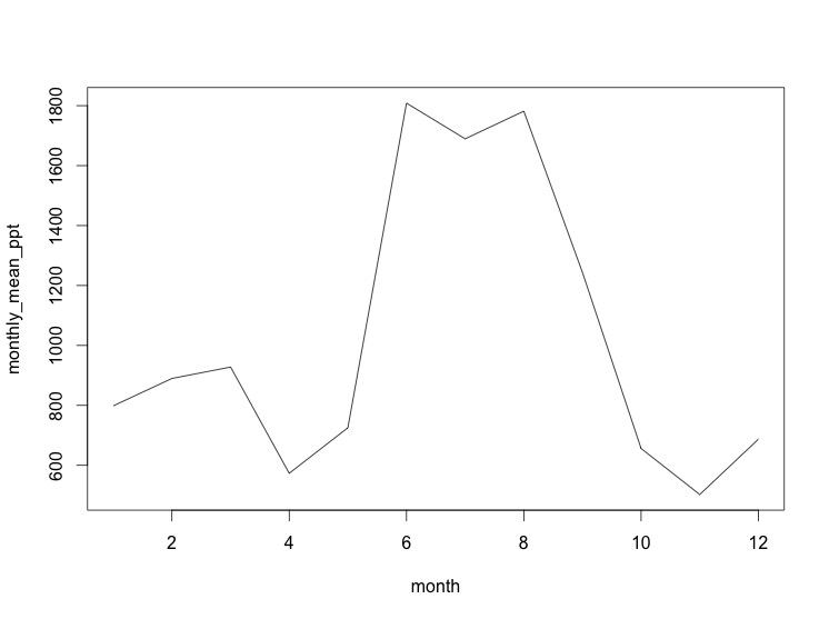
We are interested in understanding the monthly variation in precipitation in Gainesville, FL. We’ll use some data from the NOAA National Climatic Data Center.

Each row of the data file is a year (from 1961-2013) and each column is a month (January - December).

Rearrange the following program so that it:
- Imports the data
- Calculates the average precipitation in each month across years
- Plots the monthly averages as a simple line plot
Finally, add a comment above the code that describes what it does. The comment character in R is #.

It’s OK if you don’t know exactly how the details of the program work at this point, you just need to figure out the right order of the lines based on when variables are defined and when they are used.
```
plot(monthly_mean_ppt, type = "l", xlab = "Month", ylab = "Mean Precipitation")
monthly_mean_ppt <- colMeans(ppt_data)
ppt_data <- read.csv("https://datacarpentry.org/semester-biology/data/gainesville-precip.csv", header = FALSE)
```
[click here for output]
Bird Banding (15 pts)

The number of birds banded at a series of sampling sites has been counted by your field crew and entered into the following vector. Counts are entered in order and sites are numbered starting at one. Cut and paste the vector into your assignment and then answer the following questions by printing them to the screen. Some R functions that will come in handy include length(), max(), min(), sum(), and mean().
```
number_of_birds <- c(28, 32, 1, 0, 10, 22, 30, 19, 145, 27, 
36, 25, 9, 38, 21, 12, 122, 87, 36, 3, 0, 5, 55, 62, 98, 32, 
900, 33, 14, 39, 56, 81, 29, 38, 1, 0, 143, 37, 98, 77, 92, 
83, 34, 98, 40, 45, 51, 17, 22, 37, 48, 38, 91, 73, 54, 46,
102, 273, 600, 10, 11)
```
1. How many sites are there?
2. How many birds were counted at site 42?
3. What is the total number of birds counted across all of the sites?
4. What is the smallest number of birds counted?
5. What is the largest number of birds counted?
6. What is the average number of birds seen at a site?
7. How many birds were counted at the last site? Have the computer choose the last site automatically in some way, not by manually entering its position. Do you know a function that will give you the position of the last value? (since positions start at 1 the position of the last value in a vector is the same as its length).
[click here for output]
Shrub Volume Vectors (10 pts)

You have data on the length, width, and height of 10 individuals of the yew Taxus baccata stored in the following vectors:
```
length <- c(2.2, 2.1, 2.7, 3.0, 3.1, 2.5, 1.9, 1.1, 3.5, 2.9)
width <- c(1.3, 2.2, 1.5, 4.5, 3.1, NA, 1.8, 0.5, 2.0, 2.7)
height <- c(9.6, 7.6, 2.2, 1.5, 4.0, 3.0, 4.5, 2.3, 7.5, 3.2)
```
Copy these vectors into an R script and then determine the following:
1. The volume of each shrub (i.e., the length times the width times the height). storing this in a variable will make some of the next problems easier
2. The total volume of all of the shrubs.
3. A vector of the height of shrubs with lengths greater than 2.5.
4. A vector of the height of shrubs with heights greater than 5.
5. A vector of the heights of the first 5 shrubs.
6. A vector of the volumes of the first 3 shrubs.
Challenge: A vector of the volumes of the last 5 shrubs with the code written so that it will return the last 5 values regardless of the length of the vector (i.e., it will give the last 5 values if their are 10, 20, or 50 individuals).
[click here for output]
Shrub Volume Data Frame (15 pts)

This is a follow up to Shrub Volume Vectors.

One of your collaborators has posted a comma-delimited text file online for you to analyze. The file contains dimensions of a series of shrubs (shrubID, length, width, height) and they need you to determine their volumes (length * width * height). You could do this using a spreadsheet, but the project that you are working on is going to be generating lots of these files so you decide to write a program to automate the process.

Download the data, use read.csv() to import it into R, and use it to produce the following information:
1. A vector of shrub lengths
2. A vector of the volume of each of the shrubs
3. A data frame with just the shrubID and height columns
4. A data frame with the second row of the full data frame
5. A data frame with the first 5 rows of the full data frame
[click here for output]

Assignment submission & checklist

Assignment

Learning Objectives

Reading

Topics

Readings

Introduction to RStudio (choose one)

Introduction to R

Starting with Data

Lecture Notes

Exercises